Implementing Gaussian Process in Python and R
library(reticulate)
reticulate::use_condaenv("dl")
knitr::opts_chunk$set(message = F, warning = F)
This blog post is trying to implementing Gaussian Process (GP) in both Python and R. The main purpose is for my personal practice and hopefully it can also be a reference for future me and other people. In fact, it’s actually converted from my first homework in a Bayesian Deep Learning class.
All of the equations or figures mentioned in this post can be referened in the Rasmussen & Williams’ textbook for Gaussian Process.
Background
Gaussian Process (GP) can be represented in the form of
where
Mean & kernel functions
For simplicity, our mean function is set to be 0 for all x inputs.
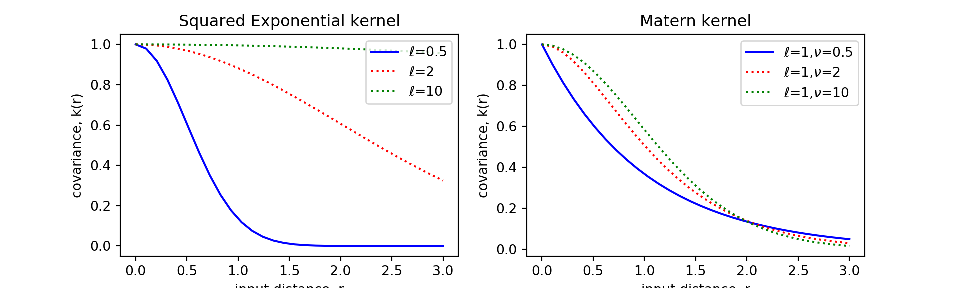
Squared Exponential kernel (Eq. 4.9)
Matern kernel (Eq. 4.14)
Implementations in Python
import numpy as np
from scipy.special import gamma, kv
import matplotlib.pyplot as plt

def mean_func(x):
    return np.zeros(len(x))

def get_r(x1, x2):
    return np.subtract.outer(x1, x2)

def sqexp_kernel(r, l = 1):
    return np.exp(-0.5 * (r/l)**2)

def matern_kernel(r, l = 1, v = 1):
    r = np.abs(r)
    r[r == 0] = 1e-8
    part1 = 2 ** (1 - v) / gamma(v)
    part2 = (np.sqrt(2 * v) * r / l) ** v
    part3 = kv(v, np.sqrt(2 * v) * r / l)
    return part1 * part2 * part3
Implementations in R
library(MASS)
library(plotly)

mean_func <- function(x) {
  rep(0, length(x))
}

get_r <- function(x1, x2) {
  outer(x1, x2, FUN = "-")
}

sqexp_kernel <- function(r, l = 1) {
  exp(-0.5 * (r/l)^2)
}

matern_kernel <- function(r, l = 1, v = 1) {
  r <- abs(r)
  r[r == 0] <- 1e-8
  part1 = 2^(1-v) / gamma(v)
  part2 = (sqrt(2*v) * r / l)^v
  part3 = besselK(sqrt(2*v) * r / l, nu = v)
  return(part1 * part2 * part3)
}
Now let’s try to recreate the input-distance to covariance figure using the functions we defined here. Our result (done in python for my homework) is the same as the figures (e.g. Figure 4.1) in the R&W textbook.
Comparing the kernel performance
Python performance
from time import process_time
x1 = np.random.rand(100)
x2 = np.random.rand(100)
start = process_time()
for i in range(50): sqexp_test = sqexp_kernel(get_r(x1, x2))
print("SE kernel for rand:" + str((process_time() - start) / 50), " s")
## SE kernel for rand:0.0006262800000000013 sstart = process_time()
for i in range(50): matern_test = matern_kernel(get_r(x1, x2))
print("Matern kernel for rand:" + str((process_time() - start) / 50), " s")## Matern kernel for rand:0.006242040000000007 sR performance
x1 = runif(100)
x2 = runif(100)
start = Sys.time()
for(i in 1:50) se_test = sqexp_kernel(get_r(x1, x2))
print(paste("SE kernel for rand:", (Sys.time() - start)/ 100, "s"))
## [1] "SE kernel for rand: 0.000436780452728271 s"start = Sys.time()
for(i in 1:50) matern_test = matern_kernel(get_r(x1, x2))
print(paste("Matern kernel for rand:", (Sys.time() - start)/ 100, "s"))## [1] "Matern kernel for rand: 0.00152798175811768 s"The results are quite comparable. I also checked the performance when it scales up, it’s still quite similar. In fact, especially for Matern kernel, when the size of the input vectors get big, I feel like it’s slightly faster to do it in R.
Sampling function
Sampling from the Prior
Implementations in Python
def sample_prior(
        x, mean_func, cov_func, cov_args = {},
        random_seed = -1, n_samples = 5):
    x_mean = mean_func(x)
    x_cov = cov_func(get_r(x, x), **cov_args)
    random_seed = int(random_seed)
    if random_seed < 0:
        prng = np.random
    else:
        prng = np.random.RandomState(random_seed)
    out = prng.multivariate_normal(x_mean, x_cov, n_samples)
    return out
Implementations in R
sample_prior <- function(
  x, mean_func, cov_func, ..., random_seed = -1, n_samples = 5
) {
  x_mean <- mean_func(x)
  x_cov <- cov_func(get_r(x, x), ...)
  random_seed <- as.integer(random_seed)
  if (random_seed > 0) set.seed(random_seed)
  return(MASS::mvrnorm(n_sample, x_mean, x_cov))
}
Let’s try to get a few samples from the prior with SE kernel at different length-scales
plt.figure(figsize = (10, 3))
x = np.linspace(-20, 20, 200)
for l_i, l in enumerate([0.25, 1.0, 4.0]):
    y = sample_prior(x, mean_func, sqexp_kernel,
                     {"l": l}, n_samples = 5)
    plt.subplot(131 + l_i)
    for i in range(5):
        plt.plot(x, y[i, :], "-", alpha = 0.3)
    plt.title("$\\ell$ = " + str(l))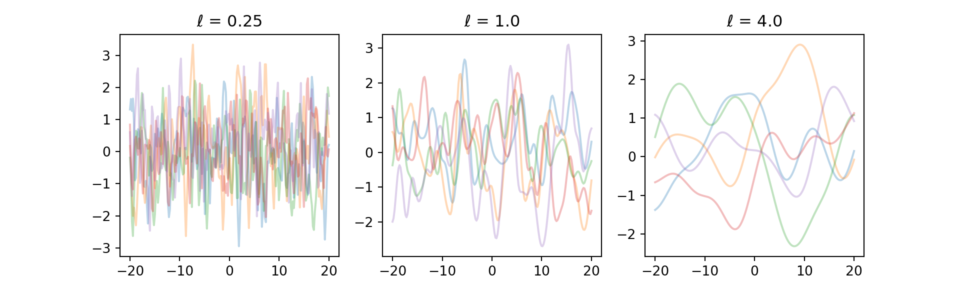
Sampling from the Posterior
Here we will implement “Prediction using Noisy Observations” because the Noise-free version can be understood as a special case of the noisy one with
Implementations in Python
def sample_posterior(
    x, y, x_star, mean_func, cov_func, cov_args = {},
    sigma_n = 0.1, random_seed = -1, n_samples = 5
):
    k_xx = cov_func(get_r(x, x), **cov_args)
    k_xxs = cov_func(get_r(x, x_star), **cov_args)
    k_xsx = cov_func(get_r(x_star, x), **cov_args)
    k_xsxs = cov_func(get_r(x_star, x_star), **cov_args)

    I = np.identity(k_xx.shape[1])
    k_xx_noise = np.linalg.inv(k_xx + sigma ** 2 * I)
    kxsx_kxxNoise = np.matmul(k_xsx, k_xx_noise)
    # Eq.2.23, 24
    fsb = np.matmul(kxsx_kxxNoise, y_train_N)
    cov_fs = k_xsxs - np.matmul(kxsx_kxxNoise, k_xxs)
    random_seed = int(random_seed)
    if random_seed < 0:
        prng = np.random
    else:
        prng = np.random.RandomState(random_seed)
    out = prng.multivariate_normal(fsb, cov_fs, n_samples)
    return out, fsb, cov_fs
Implementations in R
sample_posterior <- function(
  x, y, x_star, mean_func, cov_func, ...,
  sigma_n = 0.1, random_seed = -1, n_samples = 5
) {
  k_xx = cov_func(get_r(x, x), ...)
  k_xxs = cov_func(get_r(x, x_star), ...)
  k_xsx = cov_func(get_r(x_star, x), ...)
  k_xsxs = cov_func(get_r(x_star, x_star), ...)

  I = diag(1, dim(k_xx)[1])
  k_xx_noise = solve(k_xx + sigma_n ^ 2 * I)
  kxsx_kxxNoise = k_xsx %*% k_xx_noise
  # Eq.2.23, 24
  fsb = kxsx_kxxNoise %*% y
  cov_fs = k_xsxs - kxsx_kxxNoise %*% k_xxs
  random_seed <- as.integer(random_seed)
  if (random_seed > 0) set.seed(random_seed)
  return(MASS::mvrnorm(n_samples, fsb, cov_fs))
}
This time let’s try to fit some points in R.
x_train <- c(-10, -8, -5, 3, 7, 15)
y_train <- c(-5, -2, 3, 3, 2, 5)
x_star <- seq(-20, 20, length = 200)

par(mfrow = c(3, 3))
l <- c(0.25, 1, 4)
v <- c(0.5, 2, 8)
for (i in seq(length(l))) {
  for (j in seq(length(v))) {
    dt <- sample_posterior(
      x_train, y_train, x_star, mean_func, matern_kernel,
      l = l[i], v = v[j], n_samples = 10, random_seed = 100
    )
    matplot(x_star, t(dt), "l", col = rgb(0.3, 0.3, 0.3, 0.3), lty = 1,
            main = paste("l=", l[i], ",v=", v[j]), ylim = c(-8, 8),
            xlab = "x", ylab = "y")
    points(x = x_train, y = y_train, pch = 16, col = "red")
  }
}
Note, that when y.